#!/usr/bin/env python
# coding: utf-8
# # Machine Learning with Python
#
# Collaboratory workshop
#
# This is a notebook developed for the third day of the Collaboratory Workshop, Machine Learning with Python. For more information, go to the workshop home page:
#
# https://github.com/kose-y/W17.MachineLearning/wiki/Day-3
# - __Day 1__ - Fundamentals and Motivation
# - __Day 2__ - Classification and Cross-Validation
# - __Day 3__ - Regression and Unsupervised Learning
# - Linear and nonlinear regressions
# - Unsupervised learning
# - Conclusions
# In[ ]:
import numpy as np
import matplotlib.pyplot as plt
plt.rcParams['font.size'] = 15 # increase font size within a plot
# ## Regression
#
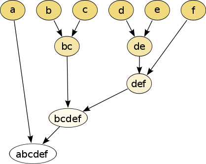
# From a set of features, determine a continuous target.
#
# e.g., Create a function that estimates the cell volume
#
#

#
#

#
#

#
#
#
 #
#
# In[ ]:
from sklearn.datasets import load_iris
# In[ ]:
iris_data = load_iris()
print( iris_data.data.shape )
# In[ ]:
iris_data.feature_names
# Before we move on, let's visualize the dataset. You can change the features being visualized below.
# In[ ]:
plt.plot( iris_data.data[:,1], iris_data.data[:,3], 'o' ) # Sepal width and Petal width.
plt.show()
# In[ ]:
plt.plot( iris_data.data[:,1], iris_data.data[:,3], 'o',
color=(0.2,0.5,1.0), markersize=4 )
plt.xlabel('Sepal width (cm)')
plt.ylabel('Petal width (cm)')
plt.tight_layout()
plt.show()
# Next, let's create a KMeans model and apply to the iris dataset. Because we know there are three different species of plants in this dataset, let's make an educated guess and use $K=3$ (i.e., we will set the parameter ```n_clusters``` to 3).
#
# https://scikit-learn.org/stable/modules/generated/sklearn.cluster.KMeans.html
# In[ ]:
from sklearn.cluster import KMeans
# In[ ]:
kmeans = KMeans( n_clusters=3 )
# In[ ]:
kmeans.fit( iris_data.data )
# After the K-means method is applied to the dataset, we can then get the ID of the clusters to which each of the samples is predicted to belong to by using the method ```predict```.
# In[ ]:
clusters = kmeans.predict( iris_data.data )
print( "Shape: ", clusters.shape )
print( "Cluster IDs: ", clusters )
# Let's visualize the resulting clustering by color-coding each cluster ID. This is very similar to how we color-coded different classes in classification datasets.
# In[ ]:
index0 = clusters == 0
index1 = clusters == 1
index2 = clusters == 2
# In[ ]:
plt.plot( iris_data.data[index0,1], iris_data.data[index0,3],
'o', color='b', markersize=4 )
plt.plot( iris_data.data[index1,1], iris_data.data[index1,3],
'o', color='k', markersize=4 )
plt.plot( iris_data.data[index2,1], iris_data.data[index2,3],
'o', color='r', markersize=4 )
plt.xlabel('Sepal width (cm)')
plt.ylabel('Petal width (cm)')
plt.show()
# Let's try $K=4$ and inspect what comes out differently.
# In[ ]:
kmeans = KMeans( n_clusters=4 )
kmeans.fit( iris_data.data )
clusters = kmeans.predict( iris_data.data )
index0 = clusters == 0
index1 = clusters == 1
index2 = clusters == 2
index3 = clusters == 3
plt.plot( iris_data.data[index0,1], iris_data.data[index0,3],
'o', color='b', markersize=4 )
plt.plot( iris_data.data[index1,1], iris_data.data[index1,3],
'o', color='k', markersize=4 )
plt.plot( iris_data.data[index2,1], iris_data.data[index2,3],
'o', color='r', markersize=4 )
plt.plot( iris_data.data[index3,1], iris_data.data[index3,3],
'o', color='g', markersize=4 )
plt.xlabel('Sepal width (cm)')
plt.ylabel('Petal width (cm)')
plt.show()
# - Because K-means assumes known number of clusters, there is some freedom. $K$ can be treated as a hyperparameter.
# - There are methodologies that do not assume the number of clusters known (e.g. affinity propagation, density-based clustering, etc.)
# - K-means is one of the simplest clustering algorithm, and might not be ideal for your application. However, some modifications (e.g. K-medians, K-means++, etc.) are still widely used.
# - When applying clustering, remember that this is different from classification: if what you need is predict categories associated to samples, use supervised learning if possible.
# ## Principal Component Analysis
# PCA can be included in the umbrella of unsupervised learning methods.
#
# - __PCA finds a set of new features that are uncorrelated among themselves__.
# - This is interesting because __correlated features overlap in what information content they include__.
# - The features are linear combination of the original features that maximally describes variations in the feature space.
# ### A little bit more detail of PCA
#
# __Covariance__: a measure of joint variability of two random variables:
#
# $$
# Cov(X, Y) = E[XY] - E[X] E[Y]
# $$
#
# - If the two variables are independent, covariance between them is zero.
# - For instance, number of people riding New York subway and probability of rain in New York have high positive covariance
#
# __Covariance Matrix__: The matrix of covariances between each pair of variables in a set. Always positive definite and symmetric
#
# __Change of basis__
#
#
#
#
# In[ ]:
from sklearn.datasets import load_iris
# In[ ]:
iris_data = load_iris()
print( iris_data.data.shape )
# In[ ]:
iris_data.feature_names
# Before we move on, let's visualize the dataset. You can change the features being visualized below.
# In[ ]:
plt.plot( iris_data.data[:,1], iris_data.data[:,3], 'o' ) # Sepal width and Petal width.
plt.show()
# In[ ]:
plt.plot( iris_data.data[:,1], iris_data.data[:,3], 'o',
color=(0.2,0.5,1.0), markersize=4 )
plt.xlabel('Sepal width (cm)')
plt.ylabel('Petal width (cm)')
plt.tight_layout()
plt.show()
# Next, let's create a KMeans model and apply to the iris dataset. Because we know there are three different species of plants in this dataset, let's make an educated guess and use $K=3$ (i.e., we will set the parameter ```n_clusters``` to 3).
#
# https://scikit-learn.org/stable/modules/generated/sklearn.cluster.KMeans.html
# In[ ]:
from sklearn.cluster import KMeans
# In[ ]:
kmeans = KMeans( n_clusters=3 )
# In[ ]:
kmeans.fit( iris_data.data )
# After the K-means method is applied to the dataset, we can then get the ID of the clusters to which each of the samples is predicted to belong to by using the method ```predict```.
# In[ ]:
clusters = kmeans.predict( iris_data.data )
print( "Shape: ", clusters.shape )
print( "Cluster IDs: ", clusters )
# Let's visualize the resulting clustering by color-coding each cluster ID. This is very similar to how we color-coded different classes in classification datasets.
# In[ ]:
index0 = clusters == 0
index1 = clusters == 1
index2 = clusters == 2
# In[ ]:
plt.plot( iris_data.data[index0,1], iris_data.data[index0,3],
'o', color='b', markersize=4 )
plt.plot( iris_data.data[index1,1], iris_data.data[index1,3],
'o', color='k', markersize=4 )
plt.plot( iris_data.data[index2,1], iris_data.data[index2,3],
'o', color='r', markersize=4 )
plt.xlabel('Sepal width (cm)')
plt.ylabel('Petal width (cm)')
plt.show()
# Let's try $K=4$ and inspect what comes out differently.
# In[ ]:
kmeans = KMeans( n_clusters=4 )
kmeans.fit( iris_data.data )
clusters = kmeans.predict( iris_data.data )
index0 = clusters == 0
index1 = clusters == 1
index2 = clusters == 2
index3 = clusters == 3
plt.plot( iris_data.data[index0,1], iris_data.data[index0,3],
'o', color='b', markersize=4 )
plt.plot( iris_data.data[index1,1], iris_data.data[index1,3],
'o', color='k', markersize=4 )
plt.plot( iris_data.data[index2,1], iris_data.data[index2,3],
'o', color='r', markersize=4 )
plt.plot( iris_data.data[index3,1], iris_data.data[index3,3],
'o', color='g', markersize=4 )
plt.xlabel('Sepal width (cm)')
plt.ylabel('Petal width (cm)')
plt.show()
# - Because K-means assumes known number of clusters, there is some freedom. $K$ can be treated as a hyperparameter.
# - There are methodologies that do not assume the number of clusters known (e.g. affinity propagation, density-based clustering, etc.)
# - K-means is one of the simplest clustering algorithm, and might not be ideal for your application. However, some modifications (e.g. K-medians, K-means++, etc.) are still widely used.
# - When applying clustering, remember that this is different from classification: if what you need is predict categories associated to samples, use supervised learning if possible.
# ## Principal Component Analysis
# PCA can be included in the umbrella of unsupervised learning methods.
#
# - __PCA finds a set of new features that are uncorrelated among themselves__.
# - This is interesting because __correlated features overlap in what information content they include__.
# - The features are linear combination of the original features that maximally describes variations in the feature space.
# ### A little bit more detail of PCA
#
# __Covariance__: a measure of joint variability of two random variables:
#
# $$
# Cov(X, Y) = E[XY] - E[X] E[Y]
# $$
#
# - If the two variables are independent, covariance between them is zero.
# - For instance, number of people riding New York subway and probability of rain in New York have high positive covariance
#
# __Covariance Matrix__: The matrix of covariances between each pair of variables in a set. Always positive definite and symmetric
#
# __Change of basis__
#
#  #
#
# The new covariance matrix is diagonal, new basis are orthogonal from each other. i.e., uncorrelated.
#
# https://scikit-learn.org/stable/modules/generated/sklearn.decomposition.PCA.html
# Let's see PCA in action by creating three variables with correlation:
# In[ ]:
from sklearn.decomposition import PCA
# In[ ]:
# 200 samples with 3 features
X = np.random.random( (200, 3) )
X[:,2] = X[:,0] # First and last features are perfectly corrleated
# numpy's cov function assumes each row to be each variable, so we transpose it.
#
# In[ ]:
# \n breaks the line
print("Covariance matrix:\n ", np.cov(X.T))
# In[ ]:
# np.cov expects the input to be a (number of features) x (number of samples) matrix.
plt.matshow(np.cov(X.T))
plt.show()
# ### Applying the PCA transformation
# In[ ]:
pca = PCA()
pca.fit(X)
# Proportions of variance explained by each principal component. Because two of the features were perfectly correlated, it is expected to have first two PCs explains most of the variance.
# In[ ]:
pca.explained_variance_ratio_
# In[ ]:
pca.components_ # Each column is the principal component
# The PC with highest variance includes variables 0 and 2; and the second PC mostly includes variable 1.
# The transformation computes the coordinated based on the changed basis
# In[ ]:
X_transform = pca.transform(X)
print(np.cov(X_transform.T))
plt.matshow(np.cov(X_transform.T))
plt.savefig('CovMatrix_example_PCA.png', dpi=300)
plt.show()
# No off-diagonal elements, almost no self-correlation for the last variable.
# ## Using PCA on the Breast Cancer dataset
# Let's apply PCA to the Breast cancer dataset from Day 1:
# In[ ]:
from sklearn.datasets import load_breast_cancer
bcancer = load_breast_cancer()
# We split the data into training and test datasets.
# In[ ]:
X, X_test, Y, Y_test = train_test_split(
bcancer.data,bcancer.target,test_size=0.2,
shuffle=False)
# In[ ]:
pca = PCA()
pca.fit( X )
# Let's visualize the importance of each Principal Component.
# In[ ]:
plt.plot( pca.explained_variance_ratio_, 'o--' )
plt.ylabel( 'Explained Variance' )
plt.xlabel( 'Principal Component #' )
plt.show()
# A better way to visualize the decay is using log-scale:
# In[ ]:
plt.plot( pca.explained_variance_ratio_, 'o--' )
plt.ylabel( 'Explained Variance' )
plt.yscale('log')
plt.xlabel( 'Principal Component #' )
plt.show()
# In[ ]:
pca.explained_variance_ratio_
# As a __dimensionality reduction__, we can choose only the first two principal components. We can apply any other machine learning methods we learned in this workshop on the data with the reduced dimension:
# In[ ]:
X_PCAs = pca.transform( X )
index0 = (Y == 0)
index1 = (Y == 1)
plt.plot( X_PCAs[index0,0],
X_PCAs[index0,1], 's', color='r' ) # malignant
plt.plot( X_PCAs[index1,0],
X_PCAs[index1,1], 'o', color='b' ) # benign
plt.xlabel('PC 1')
plt.ylabel('PC 2')
plt.show()
# We can fit random forest classifier on the transformed two-dimensional features:
# In[ ]:
from sklearn.ensemble import RandomForestClassifier
clf = RandomForestClassifier(n_estimators = 100, max_depth = 5)
clf.fit(X_PCAs[:, :2],Y)
X_test_PCAs = pca.transform( X_test )
clf.score(X_test_PCAs[:,:2],Y_test)
# We still get an OK result with only two features. On a high-dimensional dataset such as gene expression, where the number of features is much higher than the number of samples, it often improves the results.
# ## Workshop evaluation:
# (shown in the classroom)
#
#
#
# ## Concluding Remarks
#
# - We extensively explored __Jupyter Notebook__
# - We explored useful functionalities from __NumPy__ and __Matplotlib__ libraries
# - We studied __supervised learning__ and its two fundamental sub-fields: __classification__ and __regression__.
# - We investigated __Scikit-learn__'s structure and discussed in detail how to use its documentation pages.
# - At the end, we briefly discussed __unsupervised learning__.
#
# | | | |
# |:---:|:---:|:---:|
# |
#
#
# The new covariance matrix is diagonal, new basis are orthogonal from each other. i.e., uncorrelated.
#
# https://scikit-learn.org/stable/modules/generated/sklearn.decomposition.PCA.html
# Let's see PCA in action by creating three variables with correlation:
# In[ ]:
from sklearn.decomposition import PCA
# In[ ]:
# 200 samples with 3 features
X = np.random.random( (200, 3) )
X[:,2] = X[:,0] # First and last features are perfectly corrleated
# numpy's cov function assumes each row to be each variable, so we transpose it.
#
# In[ ]:
# \n breaks the line
print("Covariance matrix:\n ", np.cov(X.T))
# In[ ]:
# np.cov expects the input to be a (number of features) x (number of samples) matrix.
plt.matshow(np.cov(X.T))
plt.show()
# ### Applying the PCA transformation
# In[ ]:
pca = PCA()
pca.fit(X)
# Proportions of variance explained by each principal component. Because two of the features were perfectly correlated, it is expected to have first two PCs explains most of the variance.
# In[ ]:
pca.explained_variance_ratio_
# In[ ]:
pca.components_ # Each column is the principal component
# The PC with highest variance includes variables 0 and 2; and the second PC mostly includes variable 1.
# The transformation computes the coordinated based on the changed basis
# In[ ]:
X_transform = pca.transform(X)
print(np.cov(X_transform.T))
plt.matshow(np.cov(X_transform.T))
plt.savefig('CovMatrix_example_PCA.png', dpi=300)
plt.show()
# No off-diagonal elements, almost no self-correlation for the last variable.
# ## Using PCA on the Breast Cancer dataset
# Let's apply PCA to the Breast cancer dataset from Day 1:
# In[ ]:
from sklearn.datasets import load_breast_cancer
bcancer = load_breast_cancer()
# We split the data into training and test datasets.
# In[ ]:
X, X_test, Y, Y_test = train_test_split(
bcancer.data,bcancer.target,test_size=0.2,
shuffle=False)
# In[ ]:
pca = PCA()
pca.fit( X )
# Let's visualize the importance of each Principal Component.
# In[ ]:
plt.plot( pca.explained_variance_ratio_, 'o--' )
plt.ylabel( 'Explained Variance' )
plt.xlabel( 'Principal Component #' )
plt.show()
# A better way to visualize the decay is using log-scale:
# In[ ]:
plt.plot( pca.explained_variance_ratio_, 'o--' )
plt.ylabel( 'Explained Variance' )
plt.yscale('log')
plt.xlabel( 'Principal Component #' )
plt.show()
# In[ ]:
pca.explained_variance_ratio_
# As a __dimensionality reduction__, we can choose only the first two principal components. We can apply any other machine learning methods we learned in this workshop on the data with the reduced dimension:
# In[ ]:
X_PCAs = pca.transform( X )
index0 = (Y == 0)
index1 = (Y == 1)
plt.plot( X_PCAs[index0,0],
X_PCAs[index0,1], 's', color='r' ) # malignant
plt.plot( X_PCAs[index1,0],
X_PCAs[index1,1], 'o', color='b' ) # benign
plt.xlabel('PC 1')
plt.ylabel('PC 2')
plt.show()
# We can fit random forest classifier on the transformed two-dimensional features:
# In[ ]:
from sklearn.ensemble import RandomForestClassifier
clf = RandomForestClassifier(n_estimators = 100, max_depth = 5)
clf.fit(X_PCAs[:, :2],Y)
X_test_PCAs = pca.transform( X_test )
clf.score(X_test_PCAs[:,:2],Y_test)
# We still get an OK result with only two features. On a high-dimensional dataset such as gene expression, where the number of features is much higher than the number of samples, it often improves the results.
# ## Workshop evaluation:
# (shown in the classroom)
#
#
#
# ## Concluding Remarks
#
# - We extensively explored __Jupyter Notebook__
# - We explored useful functionalities from __NumPy__ and __Matplotlib__ libraries
# - We studied __supervised learning__ and its two fundamental sub-fields: __classification__ and __regression__.
# - We investigated __Scikit-learn__'s structure and discussed in detail how to use its documentation pages.
# - At the end, we briefly discussed __unsupervised learning__.
#
# | | | |
# |:---:|:---:|:---:|
# | |
|  |
|  |
#
# One prominent topic we did not cover in this workshop is Neural Networks. Due to recent advancement in hardware, using multiple layers of neural networks have been massively successful in many fields, including image classification and segmentation. I believe it deserves a separate 3-day workshop with higher hardware demand (i.e. access to GPUs.)
#
# ### Some related books:
#
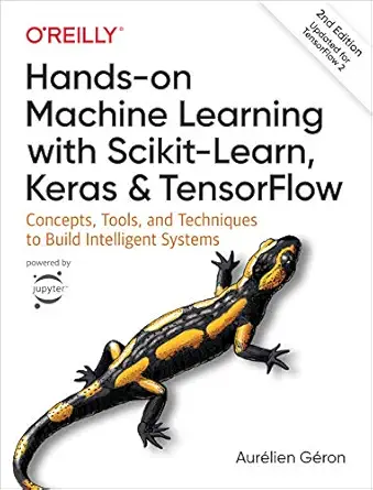
# - Hands-on Machine Learning with Scikit-Learn, Keras, and Tensorflow - Aurélien Géron (2nd ed.) : Similar approach to this workshop, with some information in deep learning with Keras and TensorFlow
#
# 
#
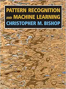
# - Pattern Recognition and Machine Learning - Christopher M. Bishop : Some mathematical approach to machine learning.
#
# 
#
# - An Introduction to Statistical Learning - Gareth James, Daniela Witten, Trevor Hastie, and Rob Tibshirani: an intro-level book for people with a bit of knowledge in math and statistics
#
# 
#
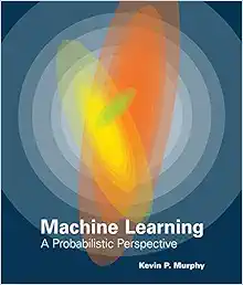
# - Machine Learning: A Probabilistic Approach - Kevin Murphy : More mathematically advanced stuff, with online software available.
#
# 
#
# - Deep Learning - Ian Goodfellow, Yoshua Bengio, and Aaron Courville
#
# 
# The goal of this workshop was
# - to provide basic information to become independent
# - increase knowledge with online resources
#
# I hope this workshop helped in this direction.
#
|
#
# One prominent topic we did not cover in this workshop is Neural Networks. Due to recent advancement in hardware, using multiple layers of neural networks have been massively successful in many fields, including image classification and segmentation. I believe it deserves a separate 3-day workshop with higher hardware demand (i.e. access to GPUs.)
#
# ### Some related books:
#
# - Hands-on Machine Learning with Scikit-Learn, Keras, and Tensorflow - Aurélien Géron (2nd ed.) : Similar approach to this workshop, with some information in deep learning with Keras and TensorFlow
#
# 
#
# - Pattern Recognition and Machine Learning - Christopher M. Bishop : Some mathematical approach to machine learning.
#
# 
#
# - An Introduction to Statistical Learning - Gareth James, Daniela Witten, Trevor Hastie, and Rob Tibshirani: an intro-level book for people with a bit of knowledge in math and statistics
#
# 
#
# - Machine Learning: A Probabilistic Approach - Kevin Murphy : More mathematically advanced stuff, with online software available.
#
# 
#
# - Deep Learning - Ian Goodfellow, Yoshua Bengio, and Aaron Courville
#
# 
# The goal of this workshop was
# - to provide basic information to become independent
# - increase knowledge with online resources
#
# I hope this workshop helped in this direction.
#
#

#
 #
#  #
#  #
#  #
#  #
#  #
#
# In[ ]:
from sklearn.datasets import load_iris
# In[ ]:
iris_data = load_iris()
print( iris_data.data.shape )
# In[ ]:
iris_data.feature_names
# Before we move on, let's visualize the dataset. You can change the features being visualized below.
# In[ ]:
plt.plot( iris_data.data[:,1], iris_data.data[:,3], 'o' ) # Sepal width and Petal width.
plt.show()
# In[ ]:
plt.plot( iris_data.data[:,1], iris_data.data[:,3], 'o',
color=(0.2,0.5,1.0), markersize=4 )
plt.xlabel('Sepal width (cm)')
plt.ylabel('Petal width (cm)')
plt.tight_layout()
plt.show()
# Next, let's create a KMeans model and apply to the iris dataset. Because we know there are three different species of plants in this dataset, let's make an educated guess and use $K=3$ (i.e., we will set the parameter ```n_clusters``` to 3).
#
# https://scikit-learn.org/stable/modules/generated/sklearn.cluster.KMeans.html
# In[ ]:
from sklearn.cluster import KMeans
# In[ ]:
kmeans = KMeans( n_clusters=3 )
# In[ ]:
kmeans.fit( iris_data.data )
# After the K-means method is applied to the dataset, we can then get the ID of the clusters to which each of the samples is predicted to belong to by using the method ```predict```.
# In[ ]:
clusters = kmeans.predict( iris_data.data )
print( "Shape: ", clusters.shape )
print( "Cluster IDs: ", clusters )
# Let's visualize the resulting clustering by color-coding each cluster ID. This is very similar to how we color-coded different classes in classification datasets.
# In[ ]:
index0 = clusters == 0
index1 = clusters == 1
index2 = clusters == 2
# In[ ]:
plt.plot( iris_data.data[index0,1], iris_data.data[index0,3],
'o', color='b', markersize=4 )
plt.plot( iris_data.data[index1,1], iris_data.data[index1,3],
'o', color='k', markersize=4 )
plt.plot( iris_data.data[index2,1], iris_data.data[index2,3],
'o', color='r', markersize=4 )
plt.xlabel('Sepal width (cm)')
plt.ylabel('Petal width (cm)')
plt.show()
# Let's try $K=4$ and inspect what comes out differently.
# In[ ]:
kmeans = KMeans( n_clusters=4 )
kmeans.fit( iris_data.data )
clusters = kmeans.predict( iris_data.data )
index0 = clusters == 0
index1 = clusters == 1
index2 = clusters == 2
index3 = clusters == 3
plt.plot( iris_data.data[index0,1], iris_data.data[index0,3],
'o', color='b', markersize=4 )
plt.plot( iris_data.data[index1,1], iris_data.data[index1,3],
'o', color='k', markersize=4 )
plt.plot( iris_data.data[index2,1], iris_data.data[index2,3],
'o', color='r', markersize=4 )
plt.plot( iris_data.data[index3,1], iris_data.data[index3,3],
'o', color='g', markersize=4 )
plt.xlabel('Sepal width (cm)')
plt.ylabel('Petal width (cm)')
plt.show()
# - Because K-means assumes known number of clusters, there is some freedom. $K$ can be treated as a hyperparameter.
# - There are methodologies that do not assume the number of clusters known (e.g. affinity propagation, density-based clustering, etc.)
# - K-means is one of the simplest clustering algorithm, and might not be ideal for your application. However, some modifications (e.g. K-medians, K-means++, etc.) are still widely used.
# - When applying clustering, remember that this is different from classification: if what you need is predict categories associated to samples, use supervised learning if possible.
# ## Principal Component Analysis
# PCA can be included in the umbrella of unsupervised learning methods.
#
# - __PCA finds a set of new features that are uncorrelated among themselves__.
# - This is interesting because __correlated features overlap in what information content they include__.
# - The features are linear combination of the original features that maximally describes variations in the feature space.
# ### A little bit more detail of PCA
#
# __Covariance__: a measure of joint variability of two random variables:
#
# $$
# Cov(X, Y) = E[XY] - E[X] E[Y]
# $$
#
# - If the two variables are independent, covariance between them is zero.
# - For instance, number of people riding New York subway and probability of rain in New York have high positive covariance
#
# __Covariance Matrix__: The matrix of covariances between each pair of variables in a set. Always positive definite and symmetric
#
# __Change of basis__
#
#
#
#
# In[ ]:
from sklearn.datasets import load_iris
# In[ ]:
iris_data = load_iris()
print( iris_data.data.shape )
# In[ ]:
iris_data.feature_names
# Before we move on, let's visualize the dataset. You can change the features being visualized below.
# In[ ]:
plt.plot( iris_data.data[:,1], iris_data.data[:,3], 'o' ) # Sepal width and Petal width.
plt.show()
# In[ ]:
plt.plot( iris_data.data[:,1], iris_data.data[:,3], 'o',
color=(0.2,0.5,1.0), markersize=4 )
plt.xlabel('Sepal width (cm)')
plt.ylabel('Petal width (cm)')
plt.tight_layout()
plt.show()
# Next, let's create a KMeans model and apply to the iris dataset. Because we know there are three different species of plants in this dataset, let's make an educated guess and use $K=3$ (i.e., we will set the parameter ```n_clusters``` to 3).
#
# https://scikit-learn.org/stable/modules/generated/sklearn.cluster.KMeans.html
# In[ ]:
from sklearn.cluster import KMeans
# In[ ]:
kmeans = KMeans( n_clusters=3 )
# In[ ]:
kmeans.fit( iris_data.data )
# After the K-means method is applied to the dataset, we can then get the ID of the clusters to which each of the samples is predicted to belong to by using the method ```predict```.
# In[ ]:
clusters = kmeans.predict( iris_data.data )
print( "Shape: ", clusters.shape )
print( "Cluster IDs: ", clusters )
# Let's visualize the resulting clustering by color-coding each cluster ID. This is very similar to how we color-coded different classes in classification datasets.
# In[ ]:
index0 = clusters == 0
index1 = clusters == 1
index2 = clusters == 2
# In[ ]:
plt.plot( iris_data.data[index0,1], iris_data.data[index0,3],
'o', color='b', markersize=4 )
plt.plot( iris_data.data[index1,1], iris_data.data[index1,3],
'o', color='k', markersize=4 )
plt.plot( iris_data.data[index2,1], iris_data.data[index2,3],
'o', color='r', markersize=4 )
plt.xlabel('Sepal width (cm)')
plt.ylabel('Petal width (cm)')
plt.show()
# Let's try $K=4$ and inspect what comes out differently.
# In[ ]:
kmeans = KMeans( n_clusters=4 )
kmeans.fit( iris_data.data )
clusters = kmeans.predict( iris_data.data )
index0 = clusters == 0
index1 = clusters == 1
index2 = clusters == 2
index3 = clusters == 3
plt.plot( iris_data.data[index0,1], iris_data.data[index0,3],
'o', color='b', markersize=4 )
plt.plot( iris_data.data[index1,1], iris_data.data[index1,3],
'o', color='k', markersize=4 )
plt.plot( iris_data.data[index2,1], iris_data.data[index2,3],
'o', color='r', markersize=4 )
plt.plot( iris_data.data[index3,1], iris_data.data[index3,3],
'o', color='g', markersize=4 )
plt.xlabel('Sepal width (cm)')
plt.ylabel('Petal width (cm)')
plt.show()
# - Because K-means assumes known number of clusters, there is some freedom. $K$ can be treated as a hyperparameter.
# - There are methodologies that do not assume the number of clusters known (e.g. affinity propagation, density-based clustering, etc.)
# - K-means is one of the simplest clustering algorithm, and might not be ideal for your application. However, some modifications (e.g. K-medians, K-means++, etc.) are still widely used.
# - When applying clustering, remember that this is different from classification: if what you need is predict categories associated to samples, use supervised learning if possible.
# ## Principal Component Analysis
# PCA can be included in the umbrella of unsupervised learning methods.
#
# - __PCA finds a set of new features that are uncorrelated among themselves__.
# - This is interesting because __correlated features overlap in what information content they include__.
# - The features are linear combination of the original features that maximally describes variations in the feature space.
# ### A little bit more detail of PCA
#
# __Covariance__: a measure of joint variability of two random variables:
#
# $$
# Cov(X, Y) = E[XY] - E[X] E[Y]
# $$
#
# - If the two variables are independent, covariance between them is zero.
# - For instance, number of people riding New York subway and probability of rain in New York have high positive covariance
#
# __Covariance Matrix__: The matrix of covariances between each pair of variables in a set. Always positive definite and symmetric
#
# __Change of basis__
#
#  #
#
# The new covariance matrix is diagonal, new basis are orthogonal from each other. i.e., uncorrelated.
#
# https://scikit-learn.org/stable/modules/generated/sklearn.decomposition.PCA.html
# Let's see PCA in action by creating three variables with correlation:
# In[ ]:
from sklearn.decomposition import PCA
# In[ ]:
# 200 samples with 3 features
X = np.random.random( (200, 3) )
X[:,2] = X[:,0] # First and last features are perfectly corrleated
# numpy's cov function assumes each row to be each variable, so we transpose it.
#
# In[ ]:
# \n breaks the line
print("Covariance matrix:\n ", np.cov(X.T))
# In[ ]:
# np.cov expects the input to be a (number of features) x (number of samples) matrix.
plt.matshow(np.cov(X.T))
plt.show()
# ### Applying the PCA transformation
# In[ ]:
pca = PCA()
pca.fit(X)
# Proportions of variance explained by each principal component. Because two of the features were perfectly correlated, it is expected to have first two PCs explains most of the variance.
# In[ ]:
pca.explained_variance_ratio_
# In[ ]:
pca.components_ # Each column is the principal component
# The PC with highest variance includes variables 0 and 2; and the second PC mostly includes variable 1.
# The transformation computes the coordinated based on the changed basis
# In[ ]:
X_transform = pca.transform(X)
print(np.cov(X_transform.T))
plt.matshow(np.cov(X_transform.T))
plt.savefig('CovMatrix_example_PCA.png', dpi=300)
plt.show()
# No off-diagonal elements, almost no self-correlation for the last variable.
# ## Using PCA on the Breast Cancer dataset
# Let's apply PCA to the Breast cancer dataset from Day 1:
# In[ ]:
from sklearn.datasets import load_breast_cancer
bcancer = load_breast_cancer()
# We split the data into training and test datasets.
# In[ ]:
X, X_test, Y, Y_test = train_test_split(
bcancer.data,bcancer.target,test_size=0.2,
shuffle=False)
# In[ ]:
pca = PCA()
pca.fit( X )
# Let's visualize the importance of each Principal Component.
# In[ ]:
plt.plot( pca.explained_variance_ratio_, 'o--' )
plt.ylabel( 'Explained Variance' )
plt.xlabel( 'Principal Component #' )
plt.show()
# A better way to visualize the decay is using log-scale:
# In[ ]:
plt.plot( pca.explained_variance_ratio_, 'o--' )
plt.ylabel( 'Explained Variance' )
plt.yscale('log')
plt.xlabel( 'Principal Component #' )
plt.show()
# In[ ]:
pca.explained_variance_ratio_
# As a __dimensionality reduction__, we can choose only the first two principal components. We can apply any other machine learning methods we learned in this workshop on the data with the reduced dimension:
# In[ ]:
X_PCAs = pca.transform( X )
index0 = (Y == 0)
index1 = (Y == 1)
plt.plot( X_PCAs[index0,0],
X_PCAs[index0,1], 's', color='r' ) # malignant
plt.plot( X_PCAs[index1,0],
X_PCAs[index1,1], 'o', color='b' ) # benign
plt.xlabel('PC 1')
plt.ylabel('PC 2')
plt.show()
# We can fit random forest classifier on the transformed two-dimensional features:
# In[ ]:
from sklearn.ensemble import RandomForestClassifier
clf = RandomForestClassifier(n_estimators = 100, max_depth = 5)
clf.fit(X_PCAs[:, :2],Y)
X_test_PCAs = pca.transform( X_test )
clf.score(X_test_PCAs[:,:2],Y_test)
# We still get an OK result with only two features. On a high-dimensional dataset such as gene expression, where the number of features is much higher than the number of samples, it often improves the results.
# ## Workshop evaluation:
# (shown in the classroom)
#
#
#
# ## Concluding Remarks
#
# - We extensively explored __Jupyter Notebook__
# - We explored useful functionalities from __NumPy__ and __Matplotlib__ libraries
# - We studied __supervised learning__ and its two fundamental sub-fields: __classification__ and __regression__.
# - We investigated __Scikit-learn__'s structure and discussed in detail how to use its documentation pages.
# - At the end, we briefly discussed __unsupervised learning__.
#
# | | | |
# |:---:|:---:|:---:|
# |
#
#
# The new covariance matrix is diagonal, new basis are orthogonal from each other. i.e., uncorrelated.
#
# https://scikit-learn.org/stable/modules/generated/sklearn.decomposition.PCA.html
# Let's see PCA in action by creating three variables with correlation:
# In[ ]:
from sklearn.decomposition import PCA
# In[ ]:
# 200 samples with 3 features
X = np.random.random( (200, 3) )
X[:,2] = X[:,0] # First and last features are perfectly corrleated
# numpy's cov function assumes each row to be each variable, so we transpose it.
#
# In[ ]:
# \n breaks the line
print("Covariance matrix:\n ", np.cov(X.T))
# In[ ]:
# np.cov expects the input to be a (number of features) x (number of samples) matrix.
plt.matshow(np.cov(X.T))
plt.show()
# ### Applying the PCA transformation
# In[ ]:
pca = PCA()
pca.fit(X)
# Proportions of variance explained by each principal component. Because two of the features were perfectly correlated, it is expected to have first two PCs explains most of the variance.
# In[ ]:
pca.explained_variance_ratio_
# In[ ]:
pca.components_ # Each column is the principal component
# The PC with highest variance includes variables 0 and 2; and the second PC mostly includes variable 1.
# The transformation computes the coordinated based on the changed basis
# In[ ]:
X_transform = pca.transform(X)
print(np.cov(X_transform.T))
plt.matshow(np.cov(X_transform.T))
plt.savefig('CovMatrix_example_PCA.png', dpi=300)
plt.show()
# No off-diagonal elements, almost no self-correlation for the last variable.
# ## Using PCA on the Breast Cancer dataset
# Let's apply PCA to the Breast cancer dataset from Day 1:
# In[ ]:
from sklearn.datasets import load_breast_cancer
bcancer = load_breast_cancer()
# We split the data into training and test datasets.
# In[ ]:
X, X_test, Y, Y_test = train_test_split(
bcancer.data,bcancer.target,test_size=0.2,
shuffle=False)
# In[ ]:
pca = PCA()
pca.fit( X )
# Let's visualize the importance of each Principal Component.
# In[ ]:
plt.plot( pca.explained_variance_ratio_, 'o--' )
plt.ylabel( 'Explained Variance' )
plt.xlabel( 'Principal Component #' )
plt.show()
# A better way to visualize the decay is using log-scale:
# In[ ]:
plt.plot( pca.explained_variance_ratio_, 'o--' )
plt.ylabel( 'Explained Variance' )
plt.yscale('log')
plt.xlabel( 'Principal Component #' )
plt.show()
# In[ ]:
pca.explained_variance_ratio_
# As a __dimensionality reduction__, we can choose only the first two principal components. We can apply any other machine learning methods we learned in this workshop on the data with the reduced dimension:
# In[ ]:
X_PCAs = pca.transform( X )
index0 = (Y == 0)
index1 = (Y == 1)
plt.plot( X_PCAs[index0,0],
X_PCAs[index0,1], 's', color='r' ) # malignant
plt.plot( X_PCAs[index1,0],
X_PCAs[index1,1], 'o', color='b' ) # benign
plt.xlabel('PC 1')
plt.ylabel('PC 2')
plt.show()
# We can fit random forest classifier on the transformed two-dimensional features:
# In[ ]:
from sklearn.ensemble import RandomForestClassifier
clf = RandomForestClassifier(n_estimators = 100, max_depth = 5)
clf.fit(X_PCAs[:, :2],Y)
X_test_PCAs = pca.transform( X_test )
clf.score(X_test_PCAs[:,:2],Y_test)
# We still get an OK result with only two features. On a high-dimensional dataset such as gene expression, where the number of features is much higher than the number of samples, it often improves the results.
# ## Workshop evaluation:
# (shown in the classroom)
#
#
#
# ## Concluding Remarks
#
# - We extensively explored __Jupyter Notebook__
# - We explored useful functionalities from __NumPy__ and __Matplotlib__ libraries
# - We studied __supervised learning__ and its two fundamental sub-fields: __classification__ and __regression__.
# - We investigated __Scikit-learn__'s structure and discussed in detail how to use its documentation pages.
# - At the end, we briefly discussed __unsupervised learning__.
#
# | | | |
# |:---:|:---:|:---:|
# | |
|  |
|  |
#
# One prominent topic we did not cover in this workshop is Neural Networks. Due to recent advancement in hardware, using multiple layers of neural networks have been massively successful in many fields, including image classification and segmentation. I believe it deserves a separate 3-day workshop with higher hardware demand (i.e. access to GPUs.)
#
# ### Some related books:
#
# - Hands-on Machine Learning with Scikit-Learn, Keras, and Tensorflow - Aurélien Géron (2nd ed.) : Similar approach to this workshop, with some information in deep learning with Keras and TensorFlow
#
# 
#
# - Pattern Recognition and Machine Learning - Christopher M. Bishop : Some mathematical approach to machine learning.
#
# 
#
# - An Introduction to Statistical Learning - Gareth James, Daniela Witten, Trevor Hastie, and Rob Tibshirani: an intro-level book for people with a bit of knowledge in math and statistics
#
# 
#
# - Machine Learning: A Probabilistic Approach - Kevin Murphy : More mathematically advanced stuff, with online software available.
#
# 
#
# - Deep Learning - Ian Goodfellow, Yoshua Bengio, and Aaron Courville
#
# 
# The goal of this workshop was
# - to provide basic information to become independent
# - increase knowledge with online resources
#
# I hope this workshop helped in this direction.
#
|
#
# One prominent topic we did not cover in this workshop is Neural Networks. Due to recent advancement in hardware, using multiple layers of neural networks have been massively successful in many fields, including image classification and segmentation. I believe it deserves a separate 3-day workshop with higher hardware demand (i.e. access to GPUs.)
#
# ### Some related books:
#
# - Hands-on Machine Learning with Scikit-Learn, Keras, and Tensorflow - Aurélien Géron (2nd ed.) : Similar approach to this workshop, with some information in deep learning with Keras and TensorFlow
#
# 
#
# - Pattern Recognition and Machine Learning - Christopher M. Bishop : Some mathematical approach to machine learning.
#
# 
#
# - An Introduction to Statistical Learning - Gareth James, Daniela Witten, Trevor Hastie, and Rob Tibshirani: an intro-level book for people with a bit of knowledge in math and statistics
#
# 
#
# - Machine Learning: A Probabilistic Approach - Kevin Murphy : More mathematically advanced stuff, with online software available.
#
# 
#
# - Deep Learning - Ian Goodfellow, Yoshua Bengio, and Aaron Courville
#
# 
# The goal of this workshop was
# - to provide basic information to become independent
# - increase knowledge with online resources
#
# I hope this workshop helped in this direction.
#  #
#